45 row labels in excel pivot table

Remove row labels from pivot table • AuditExcel.co.za Click on the Pivot table Click on the Design tab Click on the report layout button Choose either the Outline Format or the Tabular format If you like the Compact Form but want to remove 'row labels' from the Pivot Table you can also achieve it by Clicking on the Pivot Table Clicking on the Analyse tab Pivot Table "Row Labels" Header Frustration Pivot Table "Row Labels" Header Frustration. Hi Everyone please help I can't change my headers from Row Labels in a Pivot Table. Using Excel 365. Labels:

Sorting to your Pivot table row labels in custom order [quick tip] Add sort order column along with classification to the pivot table row labels area. Add the usual stuff to values area. Set up pivot table in tabular layout. Remove sub totals; Finally hide the column containing sort order. Your new pivot report is ready. Good news for people with Excel 2013 or above:

Row labels in excel pivot table

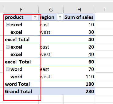
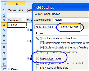
How to repeat row labels for group in pivot table? - ExtendOffice Except repeating the row labels for the entire pivot table, you can also apply the feature to a specific field in the pivot table only. 1. Firstly, you need to expand the row labels as outline form as above steps shows, and click one row label which you want to repeat in your pivot table. 2. Repeat item labels in a PivotTable - support.microsoft.com Right-click the row or column label you want to repeat, and click Field Settings. Click the Layout & Print tab, and check the Repeat item labels box. Make sure Show item labels in tabular form is selected. Notes: When you edit any of the repeated labels, the changes you make are applied to all other cells with the same label. Move Row Labels in Pivot Table - Excel Pivot Tables Move Row Labels in Pivot Table. When you add fields to the row labels area in a pivot table, the field's items are automatically sorted. See how you can manually move those labels, to put them in a different order. There's a video and written steps below. In the screen shot below, the districts are listed alphabetically, from Central to West.

Row labels in excel pivot table. How to Group Data in Pivot Table (3 Simple Methods) Following, select the PivotTable drop-down and choose the From Table/Range option. Then, select the following options in the dialog box as shown in the picture below. Step 02: Group Dates in the Pivot Table Secondly, drag the field items into the Rows and Values fields such that the table below appears. Excel 2016 Pivot table Row and Column Labels - Microsoft Community In Excel 2016 I've found when I create a pivot table it unhelpfully shows 'Row Labels' and 'Column Labels' instead of my field names, although in the top left cell it says 'Count of' and then inserts the correct field name. Years ago when I last used Excel it automatically put the field names in all three heading cells. How to Group Rows in Excel Pivot Table (3 Ways) - ExcelDemy Follow the steps below to create a PivotTable and then group the rows of dates in the table. 📌 Steps First, select anywhere in the dataset. Then, select the PivotTable icon from the Insert tab as shown in the following picture. Next, select the location for your PivotTable and then hit OK. Multiple row labels on one row in Pivot table - MrExcel Message Board I figured it out - Right click on your pivot table and choose pivot table options/display. Click on "Classic PivotTable layout" Then click on where it is subtotaling your row label and uncheck the subtotal option. D dudeshane0 New Member Joined Oct 23, 2014 Messages 1 Jan 19, 2015 #6 Gerald Higgins said:

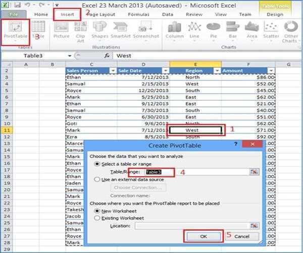
How to Use Excel Pivot Table Label Filters - Contextures Excel Tips In an Excel pivot table, you might want to hide one or more of the items in a Row field or Column field. To do that, you could click the drop down arrow for the Row or Column Labels, to see the list of pivot items in that pivot field. Then, in the list, remove the check mark for items you want to remove. Automatic Row And Column Pivot Table Labels - How To Excel At Excel The first thing to do is put your cursor somewhere in your data list Select the Insert Tab Hit Pivot Table icon Next select Pivot Table option Select a table or range option Select to put your Table on a New Worksheet or on the current one, for this tutorial select the first option Click Ok Pivot Table Row Labels - Microsoft Community If you go to PivotTable Tools > Analyze > Layout > Report Layout > Show in Tabular Form, your column headers will be used for the row labels. Every once in a while there's a sudden gust of gravity... Report abuse 1 person found this reply helpful · Was this reply helpful? Yes No A. User Replied on December 19, 2017 Pivot Table Row Labels - AuditExcel Go back to Automatic option. Right click on the Row Labels again – go to Field Settings. Look at Layout and Print. At the moment it is ticked as “show item ...

excel - Custom row labels in PivotTable - Stack Overflow 1 you can give nicknames to the fields that you are checking which populate the pivot table. If you go the pivot table data and right click you can change the value field settings to give a custom name to a row/series but I do not know about individual data points. path: pivot table data => right click => select Field Settings => edit custom name. get a row label from pivot table - Microsoft Tech Community Creating PivotTable add data to data model by checking Create PivotTable and after that convert it to cube formulas. Now you may take these formulas and convert it to form you need, for example in H3 it could be =CUBEVALUE( "ThisWorkbookDataModel", CUBEMEMBER("ThisWorkbookDataModel", " [Measures]. Pivot table row labels side by side - Excel Tutorials - OfficeTuts Excel You can copy the following table and paste it into your worksheet as Match Destination Formatting. Now, let's create a pivot table ( Insert >> Tables >> Pivot Table) and check all the values in Pivot Table Fields. Fields should look like this. Right-click inside a pivot table and choose PivotTable Options…. Check data as shown on the image below. How to make row labels on same line in pivot table? - ExtendOffice Make row labels on same line with PivotTable Options You can also go to the PivotTable Options dialog box to set an option to finish this operation. 1. Click any one cell in the pivot table, and right click to choose PivotTable Options, see screenshot: 2.

Use excel pivot table layout to add label to entry - Stack Overflow

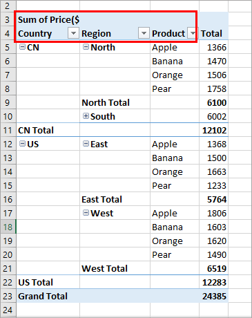
pivot table - How to extract the full row label from Excel PivotTable ... 1. I have a PivotTable in Excel with multiple layers of row filtering: Month > Region > Product (1 > EU > Dessert). When I mouse over the row, I am able to see the full row label (1 - EU - Dessert): pivot row label. I know that I can go to PivotTable Tools > Design > Report Layout > Show in Tabular Form and then Repeat All Item Labels and then ...

How to Repeat Row Labels in Pivot Table - Free Excel Tutorial

Pivot table row labels in separate columns • AuditExcel.co.za Our preference is rather that the pivot tables are shown in tabular form (all columns separated and next to each other). You can do this by changing the report format. So when you click in the Pivot Table and click on the DESIGN tab one of the options is the Report Layout. Click on this and change it to Tabular form.

Repeat Pivot Table Labels in Excel 2010 - Excel Pivot TablesExcel Pivot Tables

Changing Blank Row Labels - Excel Pivot Tables Select one of the Row or Column Labels that contains the text (blank). Type N/A in the cell, and then press the Enter key. Note: All other (Blank) items in that field will change to display the same text, N/A in this example. For more information on pivot tables, see the Pivot Table Topics on my Contextures web site.

Pivot table row labels in separate columns • AuditExcel.co.za

Design the layout and format of a PivotTable To change the layout of a PivotTable, you can change the PivotTable form and the way that fields, columns, rows, subtotals, empty cells and lines are displayed. To change the format of the PivotTable, you can apply a predefined style, banded rows, and conditional formatting. Windows Web Mac Changing the layout form of a PivotTable

EXCEL: SETTING PIVOT TABLE DEFAULTS - Strategic Finance

How to make row labels on same line in pivot table? Make row labels on same line with PivotTable Options You can also go to the PivotTable Options dialog box to set an option to finish this operation. 1. Click any one cell in the pivot table, and right click to choose PivotTable Options, see screenshot: 2.

Pivot Table Excel 2007 Repeat Row Labels | Elcho Table

How to Flatten Data in Excel Pivot Table? - GeeksforGeeks Select a range that you want to flatten - typically, a column of labels. Highlight the empty cells only - hit F5 (GoTo) and select Special > Blanks. Type equals (=) and then the Up Arrow to enter a formula with a direct cell reference to the first data label. Instead of hitting enter, hold down Control and hit Enter.

Pivot Table in Excel

Change the pivot table "Row Labels" text | MrExcel Message Board 144. Feb 4, 2021. #3. mart37 said: Click on the cell and typ the text. Thanks mart37. So simple! I was looking for a way to change it on the ribbons & settings. Typical Excel - things you think are difficult are easy, and things that should be easy are difficult!

Excel Pivot Table Combine Columns | Decoration Items Image

Formula1, Formula2 appearing as row items in pivot table where row ... if you select a row item and go to the botttom right of the cell to the black cross hairs and drag down, it inserts formula1, formula2 formula3 depend how far you dragged it, and the appear in multiple cells in the pivot table. The solution is as listed above. Going to pivot table, Analyse, Fields, items & sets, solve order and deleting the ...

MS Excel 2013: Display the fields in the Values Section in a single column in a pivot table

Use column labels from an Excel table as the rows in a Pivot Table ... Highlight your current table, including the headers Then from the Data section of the ribbon, select From Table Highlight all the columns containing data, but not the Year column, and then select Unpivot Columns Close the dialog and keep the changes. Excel should place the unpivoted data into a new worksheet, looking something like this:

Remove filter from ROW LABELS on pivot table Excel - Super User

How to rename group or row labels in Excel PivotTable? - ExtendOffice To rename Row Labels, you need to go to the Active Field textbox. 1. Click at the PivotTable, then click Analyze tab and go to the Active Field textbox. 2. Now in the Active Field textbox, the active field name is displayed, you can change it in the textbox.

excel - PivotTable to show values, not sum of values - Stack Overflow

Data Labels in Excel Pivot Chart (Detailed Analysis) Add a Pivot Chart from the PivotTable Analyze tab. Then press on the Plus right next to the Chart. Next open Format Data Labels by pressing the More options in the Data Labels. Then on the side panel, click on the Value From Cells. Next, in the dialog box, Select D5:D11, and click OK.

How to group row labels in Excel 2007 PivotTables (Excel 07-104) - YouTube

Move Row Labels in Pivot Table - Excel Pivot Tables Move Row Labels in Pivot Table. When you add fields to the row labels area in a pivot table, the field's items are automatically sorted. See how you can manually move those labels, to put them in a different order. There's a video and written steps below. In the screen shot below, the districts are listed alphabetically, from Central to West.

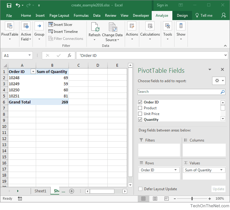
MS Excel 2016: How to Create a Pivot Table

Repeat item labels in a PivotTable - support.microsoft.com Right-click the row or column label you want to repeat, and click Field Settings. Click the Layout & Print tab, and check the Repeat item labels box. Make sure Show item labels in tabular form is selected. Notes: When you edit any of the repeated labels, the changes you make are applied to all other cells with the same label.