44 how to add horizontal labels in excel graph

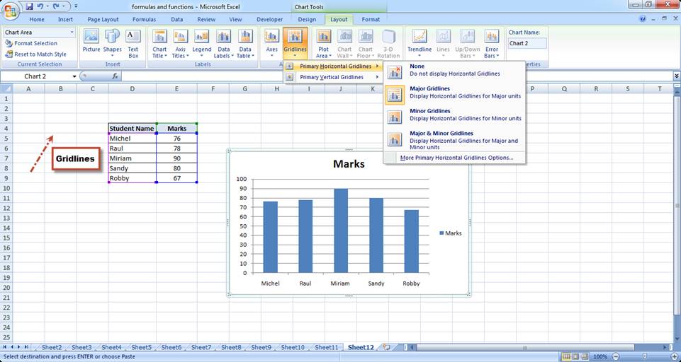
How to Add Axis Labels in Microsoft Excel - Appuals.com Click on the Chart Elements button (represented by a green + sign) next to the upper-right corner of the selected chart. Enable Axis Titles by checking the checkbox located directly beside the Axis Titles option. Once you do so, Excel will add labels for the primary horizontal and primary vertical axes to the chart. How to Create and Customize a Pareto Chart in Microsoft Excel Go to the Insert tab and click the "Insert Statistical Chart" drop-down arrow. Select "Pareto" in the Histogram section of the menu. Remember, a Pareto chart is a sorted histogram chart. And just like that, a Pareto chart pops into your spreadsheet. You'll see your categories as the horizontal axis and your numbers as the vertical axis.

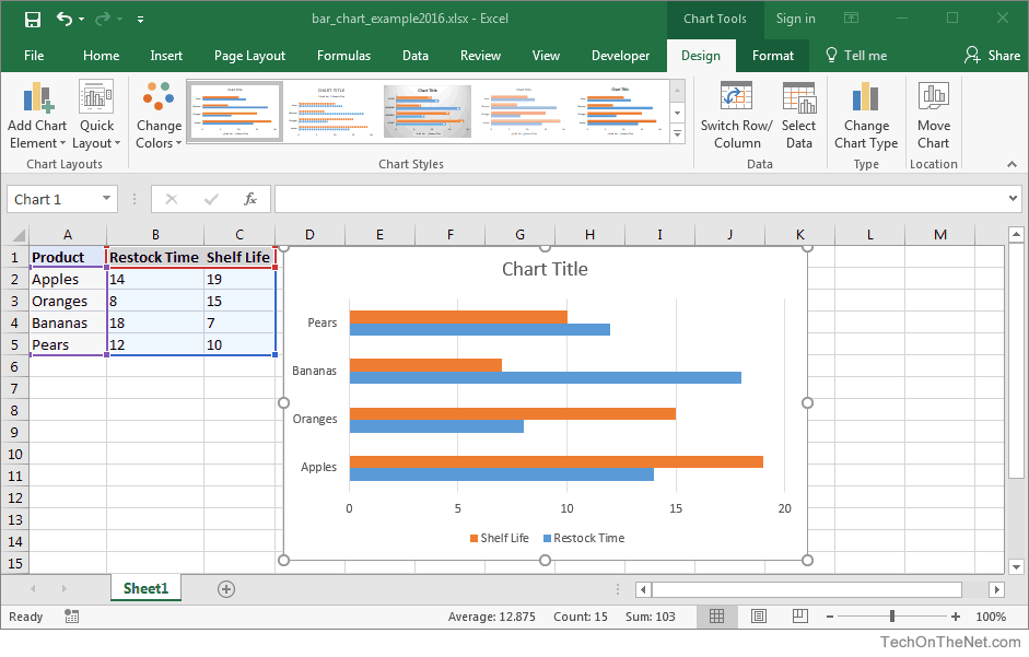
How to Create a Bar Chart in Excel with Multiple Bars? To fine tune the bar chart in excel, you can add a title to the graph. You can also add data labels. To add data labels, go to the Chart Design ribbon, and from the Add Chart Element, options select Add Data Labels. Adding data labels will add an extra flair to your graph. You can compare the score more easily and come to a conclusion faster.

How to add horizontal labels in excel graph

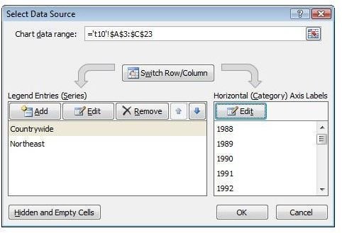
How to Select Data for Graphs in Excel - Sheetaki Select the blank graph and navigate to the Chart Design tab. Click on the Select Data option. In the Select Data Source dialog box, select the Chart data range text box and type in your range. You may also use your cursor to select the range much faster. Click on the OK button to apply the new data source to your graph. How to format axis labels individually in Excel - SpreadsheetWeb Double-click on the axis you want to format. Double-clicking opens the right panel where you can format your axis. Open the Axis Options section if it isn't active. You can find the number formatting selection under Number section. Select Custom item in the Category list. Type your code into the Format Code box and click Add button. How to Add X and Y Axis Labels in Excel (2 Easy Methods) Then go to Add Chart Element and press on the Axis Titles. Moreover, select Primary Horizontal to label the horizontal axis. In short: Select graph > Chart Design > Add Chart Element > Axis Titles > Primary Horizontal. Afterward, if you have followed all steps properly, then the Axis Title option will come under the horizontal line.

How to add horizontal labels in excel graph. How to add text labels on Excel scatter chart axis Add dummy series to the scatter plot and add data labels. 4. Select recently added labels and press Ctrl + 1 to edit them. Add custom data labels from the column "X axis labels". Use "Values from Cells" like in this other post and remove values related to the actual dummy series. Change the label position below data points. Excel Add Axis Label on Mac | WPS Office Academy 1. First, select the graph you want to add to the axis label so you can carry out this process correctly. 2. You need to navigate to where the Chart Tools Layout tab is and click where Axis Titles is. 3. You can excel add a horizontal axis label by clicking through Main Horizontal Axis Title under the Axis Title dropdown menu. Excel: How to Create a Bubble Chart with Labels - Statology To add labels to the bubble chart, click anywhere on the chart and then click the green plus "+" sign in the top right corner. Then click the arrow next to Data Labels and then click More Options in the dropdown menu: In the panel that appears on the right side of the screen, check the box next to Value From Cells within the Label Options ... How to add label to axis in excel chart on mac - WPS Office 1. After choosing your chart, go to the Chart Design tab that appears. Axis Titles will appear when you choose them with the drop-down arrow next to Add Chart Element. Choose Primary Horizontal, Primary Vertical, or both from the pop-out menu. 2. The Chart Elements icon is located to the right of the chart in Excel for Windows.

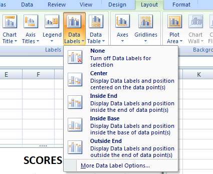
How to Create A Timeline Graph in Excel [Tutorial & Templates] - Preceden Select Series 2 (the orange line on the horizontal axis). Go to Chart tools, Design on the ribbon. On the top left, click Add Chart Element, then down to Data Labels followed by More Data Label Options. This opens the sidebar to format the data labels. Click Label Options and select Category Name under Label Contains. Change Label Position to ... Add Horizontal Line to Excel Chart - Excel Tutorials - OfficeTuts Excel Add Horizontal Line to Clustered Column To show the addition of the horizontal line, we will use Clustered Column chart, as this chart is one of the most widely used ones. We will create it based on the data of NBA players and their points in one night of basketball: How to Add Two Data Labels in Excel Chart (with Easy Steps) Table of Contents hide. Download Practice Workbook. 4 Quick Steps to Add Two Data Labels in Excel Chart. Step 1: Create a Chart to Represent Data. Step 2: Add 1st Data Label in Excel Chart. Step 3: Apply 2nd Data Label in Excel Chart. Step 4: Format Data Labels to Show Two Data Labels. Things to Remember. A Step-by-Step Guide on How to Make a Graph in Excel - Simplilearn.com How to Make a Graph in Excel You must select the data for which a chart is to be created. In the INSERT menu, select Recommended Charts. Choose any chart from the list of charts Excel recommends for your data on the Recommended Charts tab, and click it to preview how it will look with your data.

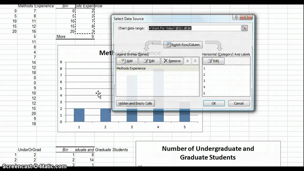
Use defined names to automatically update a chart range - Office On the Insert tab, click a chart, and then click a chart type. Click the Design tab, click the Select Data in the Data group. Under Legend Entries (Series), click Edit. In the Series values box, type =Sheet1!Sales, and then click OK. Under Horizontal (Category) Axis Labels, click Edit. In the Axis label range box, type =Sheet1!Date, and then ... Chart.Axes method (Excel) | Microsoft Docs This example adds an axis label to the category axis on Chart1. VB Copy With Charts ("Chart1").Axes (xlCategory) .HasTitle = True .AxisTitle.Text = "July Sales" End With This example turns off major gridlines for the category axis on Chart1. VB Copy Charts ("Chart1").Axes (xlCategory).HasMajorGridlines = False Excel horizontal bar graph - AislingRona The bar in the graph have to have data labels correlated to them with both. Progress Bar In Excel Cells Progress Bar Progress Excel I dont want all the bars to start at point 0.. The bars for the average values will be added to the chart. ... How To Add Horizontal Line To Excel Chart Using Best Practices Chart Graphing Line Graphs Chart does not show correct horizontal axis labels Chart does not show correct horizontal axis labels. The horizontal axis labels on my chart are replaced by running numbers from 0 to 12. When I try to select data for that axis, the edit button is greyed out. I believe, the problem is that my labels are not years but half years (custom), so the system dies not recognize them as valid points in ...

how to add data labels into Excel graphs — storytelling with data

Horizontal axis labels on a chart - Microsoft Community If you start with Jan or January, then fill down, Excel should automatically fill in the following names. Click on the chart. Click 'Select Data' on the 'Chart Design' tab of the ribbon. Click Edit under 'Horizontal (Category) Axis Labels'. Point to the range with the months, then OK your way out. --- Kind regards, HansV

Basic Excel Chart Formatting - MS Excel Charting Tutorial Part 4 | Vertical Horizons

How to make shading on Excel chart and move x axis labels to the bottom ... For the yellow shading, add a series with constant value -80, and a series with constant value -20. In the Change Chart Type dialog, change the chart type for the new series to Stacked Area. Change the color from whatever Excel decides to yellow. Finally, remove the new series form the legend. See the attached version.

How to Label Axes in Excel: 6 Steps (with Pictures) - wikiHow

Format Chart Axis in Excel - Axis Options Analyzing Format Axis Pane. Right-click on the Vertical Axis of this chart and select the "Format Axis" option from the shortcut menu. This will open up the format axis pane at the right of your excel interface. Thereafter, Axis options and Text options are the two sub panes of the format axis pane.

Excel Version 16 For Mac Adding Graph Labels - fasrtune

Modifying Axis Scale Labels (Microsoft Excel) - tips Follow these steps: Create your chart as you normally would. Double-click the axis you want to scale. You should see the Format Axis dialog box. (If double-clicking doesn't work, right-click the axis and choose Format Axis from the resulting Context menu.) Make sure the Number tab is displayed. (See Figure 1.) Figure 1.

Changing X-Axis Values - YouTube

How to Add Total Values to Stacked Bar Chart in Excel Step 4: Add Total Values. Next, right click on the yellow line and click Add Data Labels. Next, double click on any of the labels. In the new panel that appears, check the button next to Above for the Label Position: Next, double click on the yellow line in the chart. In the new panel that appears, check the button next to No line:

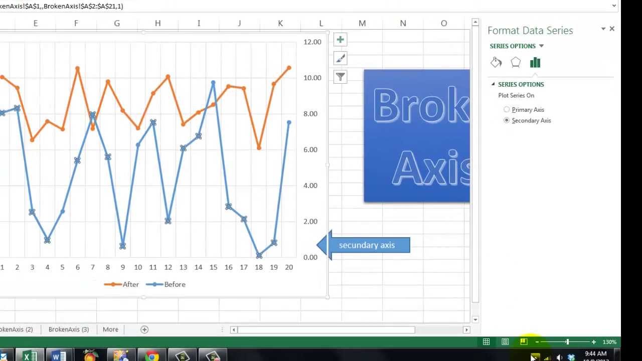
Does Excel Have a Broken Axis? - YouTube

How to Create a Mekko Chart (Marimekko) in Excel - Quick Guide Here are the steps to create a Mekko chart: #1: Set up a helper table and add data. #2: Append the helper table with zeros. #3: Apply a custom number format. #4: Calculate and add segment values. #5: Set up the horizontal axis values. #6: Calculate midpoints. #7: Add labels for rows and columns.

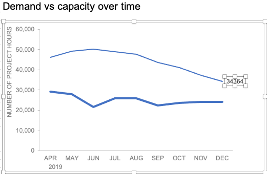
storytelling with data: plotting a value within a range

How to move Excel chart axis labels to the bottom or top - Data Cornering Move Excel chart axis labels to the bottom in 2 easy steps. Select horizontal axis labels and press Ctrl + 1 to open the formatting pane. Open the Labels section and choose label position " Low ". Here is the result with Excel chart axis labels at the bottom. Now it is possible to clearly evaluate the dynamics of the series and see axis labels.

Create a line chart with bands [tutorial] | Chandoo.org - Learn Microsoft Excel Online

How to Add Axis Titles in a Microsoft Excel Chart - How-To Geek Select your chart and then head to the Chart Design tab that displays. Click the Add Chart Element drop-down arrow and move your cursor to Axis Titles. In the pop-out menu, select "Primary Horizontal," "Primary Vertical," or both. If you're using Excel on Windows, you can also use the Chart Elements icon on the right of the chart.

Excel - 2-D Bar Chart - Change horizontal axis labels - Super User

How to Change the X-Axis in Excel - Alphr Open the Excel file and select your graph. Now, right-click on the Horizontal Axis and choose Format Axis… from the menu. Select Axis Options > Labels. Under Interval between labels, select the...

how to make a excel graph.

How To Add a Target Line in Excel (Using Two Different Methods) Use the following steps to add a target line in your Excel spreadsheet by adding a new data series: 1. Open your Excel spreadsheet To add a target line in Excel, first, open the program on your device. Then create a new spreadsheet by clicking "New." You also can open an existing one with the data you want to use for your bar graph. 2.

How to Change Labels for a Chart Axis in Excel 2007

How to Add X and Y Axis Labels in Excel (2 Easy Methods) Then go to Add Chart Element and press on the Axis Titles. Moreover, select Primary Horizontal to label the horizontal axis. In short: Select graph > Chart Design > Add Chart Element > Axis Titles > Primary Horizontal. Afterward, if you have followed all steps properly, then the Axis Title option will come under the horizontal line.

Excel Help: Making Pyramid Graph for Headcount Distribution Representation

How to format axis labels individually in Excel - SpreadsheetWeb Double-click on the axis you want to format. Double-clicking opens the right panel where you can format your axis. Open the Axis Options section if it isn't active. You can find the number formatting selection under Number section. Select Custom item in the Category list. Type your code into the Format Code box and click Add button.