44 change data labels in excel chart
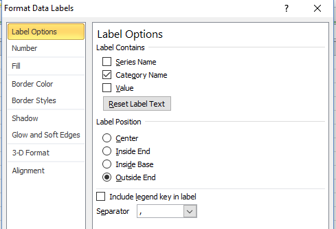
Add or remove data labels in a chart - support.microsoft.com In the upper right corner, next to the chart, click Add Chart Element > Data Labels. To change the location, click the arrow, and choose an option. If you want to show your data label inside a text bubble shape, click Data Callout. To make data labels easier to read, you can move them inside the data points or even outside of the chart. Add data labels and callouts to charts in Excel 365 - EasyTweaks.com Excel also gives you the option of formatting the data labels to suit your desired look if you don't like the default. To make changes to the data labels, right-click within the chart and select the "Format Labels" option. Some of the formatting options you will have include; changing the label position, changing its alignment angle, and many more.
How to Use Cell Values for Excel Chart Labels - How-To Geek Select the chart, choose the "Chart Elements" option, click the "Data Labels" arrow, and then "More Options." Uncheck the "Value" box and check the "Value From Cells" box. Select cells C2:C6 to use for the data label range and then click the "OK" button. The values from these cells are now used for the chart data labels.

Change data labels in excel chart
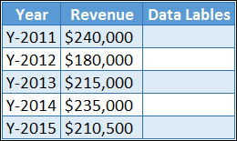
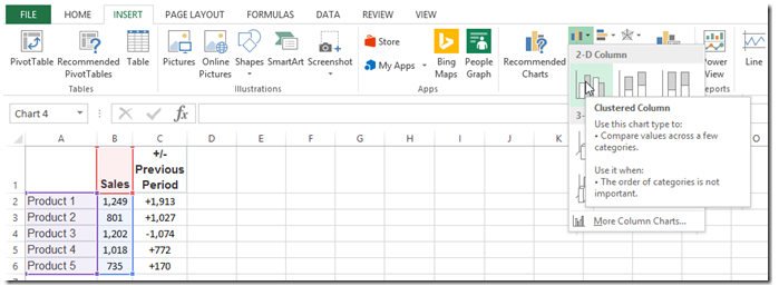
Create Dynamic Chart Data Labels with Slicers - Excel Campus Step 6: Setup the Pivot Table and Slicer. The final step is to make the data labels interactive. We do this with a pivot table and slicer. The source data for the pivot table is the Table on the left side in the image below. This table contains the three options for the different data labels. How to change chart axis labels' font color and size in Excel? Sometimes, you may want to change labels' font color by positive/negative/ in an axis in chart. You can get it done with conditional formatting easily as follows: 1. Right click the axis you will change labels by positive/negative/0, and select the Format Axis from right-clicking menu. 2. How to change Layout and Chart Style in Excel Follow the steps below to change the Chart Type in Excel: Select the Chart, then click the Change Chart Type button in the Type group on the Chart Design tab. A Change Chart Type dialog box will open.
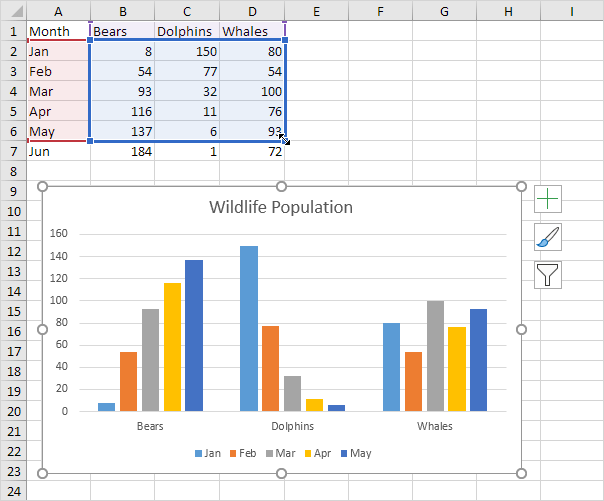
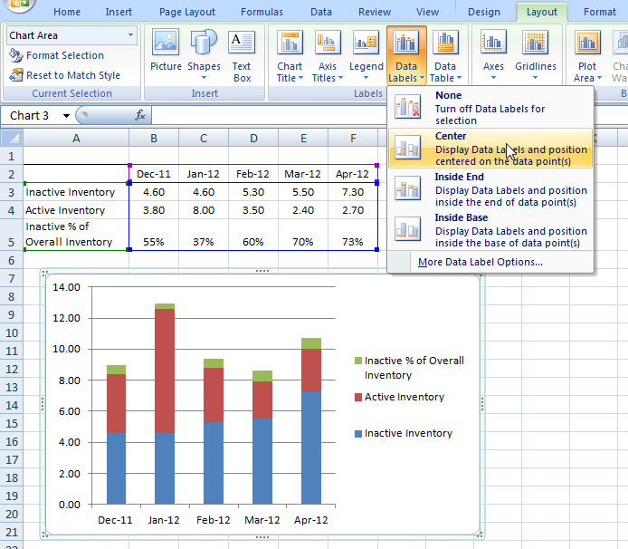
Change data labels in excel chart. Move data labels - support.microsoft.com Click any data label once to select all of them, or double-click a specific data label you want to move. Right-click the selection > Chart Elements > Data Labels arrow, and select the placement option you want. Different options are available for different chart types. Data Labels in Excel Pivot Chart (Detailed Analysis) Before adding the Data Labels, we need to create the Pivot Chart in the beginning. We can create a Pivot Chart from the Insert tab. To do this, go to Insert tab > Tables group. Then in the dialog box, select the range of cells of the primary dataset., here the range of cells is B4:J23. And select the New Worksheet in the next option. How to Customize Your Excel Pivot Chart Data Labels - dummies The Data Labels command on the Design tab's Add Chart Element menu in Excel allows you to label data markers with values from your pivot table. When you click the command button, Excel displays a menu with commands corresponding to locations for the data labels: None, Center, Left, Right, Above, and Below. None signifies that no data labels ... Add / Move Data Labels in Charts - Excel & Google Sheets Check Data Labels . Change Position of Data Labels. Click on the arrow next to Data Labels to change the position of where the labels are in relation to the bar chart. Final Graph with Data Labels. After moving the data labels to the Center in this example, the graph is able to give more information about each of the X Axis Series.
How to create Custom Data Labels in Excel Charts - Efficiency 365 Create the chart as usual. Add default data labels. Click on each unwanted label (using slow double click) and delete it. Select each item where you want the custom label one at a time. Press F2 to move focus to the Formula editing box. Type the equal to sign. Now click on the cell which contains the appropriate label. How to add data labels from different column in an Excel chart? Click any data label to select all data labels, and then click the specified data label to select it only in the chart. 3. Go to the formula bar, type =, select the corresponding cell in the different column, and press the Enter key. See screenshot: 4. Repeat the above 2 - 3 steps to add data labels from the different column for other data points. How to change Axis labels in Excel Chart - A Complete Guide Type any number in the " Distance from axis " box to change the position of the axis labels. Number Under Axis Options, click Number, and select the number format you want in the Category box. You can specify the decimal number in the Decimal places box, also you can separate 1000 using (,) and select the negative number format. How to Edit Chart Data in Excel (5 Suitable Examples) 5 Suitable Examples to Edit Chart Data in Excel 1. Modify Chart Data in Excel 2. Add New Values to Chart Data 3. Remove Values from Chart Data 4. Add New Rows to Chart Data 5. Remove Rows from Chart Data Conclusion Related Articles Download Practice Workbook You can download the workbook used to demonstrate all of the methods and examples below.
How to Change Excel Chart Data Labels to Custom Values? - Chandoo.org You can change data labels and point them to different cells using this little trick. First add data labels to the chart (Layout Ribbon > Data Labels) Define the new data label values in a bunch of cells, like this: Now, click on any data label. This will select "all" data labels. Now click once again. How to add or move data labels in Excel chart? - ExtendOffice In Excel 2013 or 2016. 1. Click the chart to show the Chart Elements button . 2. Then click the Chart Elements, and check Data Labels, then you can click the arrow to choose an option about the data labels in the sub menu. See screenshot: In Excel 2010 or 2007. 1. click on the chart to show the Layout tab in the Chart Tools group. See ... 4 Feb 2021 — 1/ Select A1:B7 > Inser your Histo. chart · 2/ Right-click i.e. on the 1st histo. · 3/ Click one of the numbers that just displayed (the Format ... Custom Chart Data Labels In Excel With Formulas In the formula-bar hit = (equals), select the cell reference containing your chart label's data. In this case, the first label is in cell E2. Finally, repeat for all your chart laebls. If you are looking for a way to add custom data labels on your Excel chart, then this blog post is perfect for you.
Chart's Data Series in Excel - Easy Excel Tutorial
How to Edit Pie Chart in Excel (All Possible Modifications) Change Data Labels Position Just like the chart title, you can also change the position of data labels in a pie chart. Follow the steps below to do this. 👇 Steps: Firstly, click on the chart area. Following, click on the Chart Elements icon. Subsequently, click on the rightward arrow situated on the right side of the Data Labels option.

Excel Course: Inserting Graphs
Change the labels in an Excel data series | TechRepublic Click the Chart Wizard button in the Standard toolbar. Click Next. Click the Series tab. Click the Window Shade button in the Category (X) Axis Labels box. Select B3:D3 to select the labels in your...

Surface Chart in Excel
How to Add Data Labels in Excel - Excelchat | Excelchat In Excel 2013 and the later versions we need to do the followings; Click anywhere in the chart area to display the Chart Elements button Figure 5. Chart Elements Button Click the Chart Elements button > Select the Data Labels, then click the Arrow to choose the data labels position. Figure 6. How to Add Data Labels in Excel 2013 Figure 7.

Change Chart Data Labels : Chart Data « Chart « Microsoft Office Excel 2007 Tutorial
Change the format of data labels in a chart To get there, after adding your data labels, select the data label to format, and then click Chart Elements > Data Labels > More Options. To go to the appropriate area, click one of the four icons ( Fill & Line, Effects, Size & Properties ( Layout & Properties in Outlook or Word), or Label Options) shown here.
Create Dynamic Excel Chart Conditional Labels and Callouts
Change order of data labels in chart - Microsoft Community Replied on March 4, 2013. In reply to Ty_hell_heaven's post on March 4, 2013. The data were added in the order shown in the list before realizing that the labels could not be moved around. The order of the labels on the right should be, downward, 10, 8, 6, 4, and 2. Report abuse.
Excel Bar Charts - Clustered, Stacked - Template - Automate Excel
How to Change Chart Data Range in Excel (5 Quick Methods) - ExcelDemy 1. Using Design Tab to Change Chart Data Range in Excel. There is a built-in process in Excel for making charts under the Charts group Feature.In addition, I need a chart to see you how to change that chart data range.Here, I will use Bar Charts Feature to make a Bar Chart.The steps are given below.
Excel Dashboard Templates How-to Put Percentage Labels on Top of a Stacked Column Chart - Excel ...
Change axis labels in a chart - support.microsoft.com Right-click the category labels you want to change, and click Select Data. In the Horizontal (Category) Axis Labels box, click Edit. In the Axis label range box, enter the labels you want to use, separated by commas. For example, type Quarter 1,Quarter 2,Quarter 3,Quarter 4. Change the format of text and numbers in labels
Labeling Excel data groups - Microsoft Community
How to change axis labels order in a bar chart - Microsoft Excel 365 See more about the competition chart. To change the order of the labels on the axis, do the following: 1. Right-click the horizontal axis and click the Format Axis... in the popup menu (or double-click the axis): 2. On the Format Axis pane, on the Axis Options tab, in the Axis Options group: Under Axis position, select the Category in reverse ...

Pie Chart - PK: An Excel Expert
Question: labels in an Excel doughnut chart Open your Excel document and click on your chart. In the upper bar you will find the "Diagram Tools". Click on the "Design" tab. In the "Data" group, click the "Select data" button. In the right window you will find the "Horizontal axis label". Click on "Edit". Now enter your desired names or values for the legend.

Format Number Options for Chart Data Labels in Excel 2011 for Mac
Excel Chart Data Labels-Modifying Orientation - Microsoft Community The chart layout tab has been absorbed into other areas in Excel 2016. I cannot figure out how to change the orientation of the data labels on the axes....(tilt, horizontal, vertical). Any help is
How To Use Dynamic Data Labels To Create Interactive Excel Charts
Edit titles or data labels in a chart - support.microsoft.com In the worksheet, click the cell that contains the title or data label text that you want to change. Edit the existing contents, or type the new text or value, and then press ENTER. The changes you made automatically appear on the chart. Top of Page Reestablish the link between a title or data label and a worksheet cell

How to Create Progress Charts (Bar and Circle) in Excel - Automate Excel
How to change Layout and Chart Style in Excel Follow the steps below to change the Chart Type in Excel: Select the Chart, then click the Change Chart Type button in the Type group on the Chart Design tab. A Change Chart Type dialog box will open.
How-to Use Data Labels from a Range in an Excel Chart - Excel Dashboard Templates
How to change chart axis labels' font color and size in Excel? Sometimes, you may want to change labels' font color by positive/negative/ in an axis in chart. You can get it done with conditional formatting easily as follows: 1. Right click the axis you will change labels by positive/negative/0, and select the Format Axis from right-clicking menu. 2.

GANTT Procedure
Create Dynamic Chart Data Labels with Slicers - Excel Campus Step 6: Setup the Pivot Table and Slicer. The final step is to make the data labels interactive. We do this with a pivot table and slicer. The source data for the pivot table is the Table on the left side in the image below. This table contains the three options for the different data labels.

How to create Custom Data Labels in Excel Charts – Efficiency 365

Custom data labels in a chart | Get Digital Help - Microsoft Excel resource

How to use symbols on charts in Excel
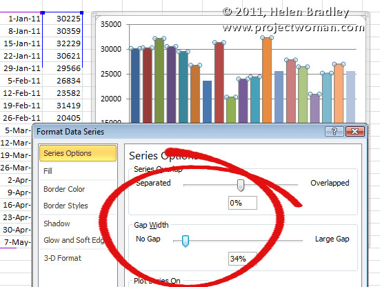
Help! My Excel Chart Columns are too Skinny « projectwoman.com
Post a Comment for "44 change data labels in excel chart"