44 how to add two data labels in excel pie chart

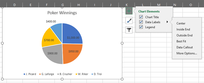
How to Make a Pie Chart with Multiple Data in Excel (2 Ways) First, to add Data Labels, click on the Plus sign as marked in the following picture. After that, check the box of Data Labels. At this stage, you will be able to see that all of your data has labels now. Next, right-click on any of the labels and select Format Data Labels. After that, a new dialogue box named Format Data Labels will pop up. How to Customize Your Excel Pivot Chart Data Labels The Data Labels command on the Design tab's Add Chart Element menu in Excel allows you to label data markers with values from your pivot table. When you click the command button, Excel displays a menu with commands corresponding to locations for the data labels: None, Center, Left, Right, Above, and Below.

Possible to add second data label to pie chart? - Excel Help Forum Re: Possible to add second data label to pie chart? Create the composite label in a worksheet column by concatenating the data in other cells and the nextline character, CHR (10). Now, use this composite label column as the source for Rob Bovey's add-in. -- Regards, Tushar Mehta Excel, PowerPoint, and VBA add-ins, tutorials

How to add two data labels in excel pie chart

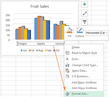
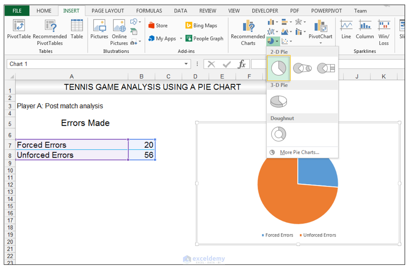
How to group (two-level) axis labels in a chart in Excel? Create a Pivot Chart with selecting the source data, and: (1) In Excel 2007 and 2010, clicking the PivotTable > PivotChart in the Tables group on the Insert Tab; (2) In Excel 2013, clicking the Pivot Chart > Pivot Chart in the Charts group on the Insert tab. 2. In the opening dialog box, check the Existing worksheet option, and then select a ... Pie Chart in Excel - Inserting, Formatting, Filters, Data Labels Click on the Instagram slice of the pie chart to select the instagram. Go to format tab. (optional step) In the Current Selection group, choose data series "hours". This will select all the slices of pie chart. Click on Format Selection Button. As a result, the Format Data Point pane opens. How to Make Multiple Pie Charts from One Table (3 Easy Ways) Afterward, go to the Insert tab >> click on Pie Charts. Then, select the 2-D Pie chart. After that, click on the "+" sign to open Chart Elements. Next, turn on Data Labels. Finally, you will get one pie chart from multiple tables in Excel. Practice Section

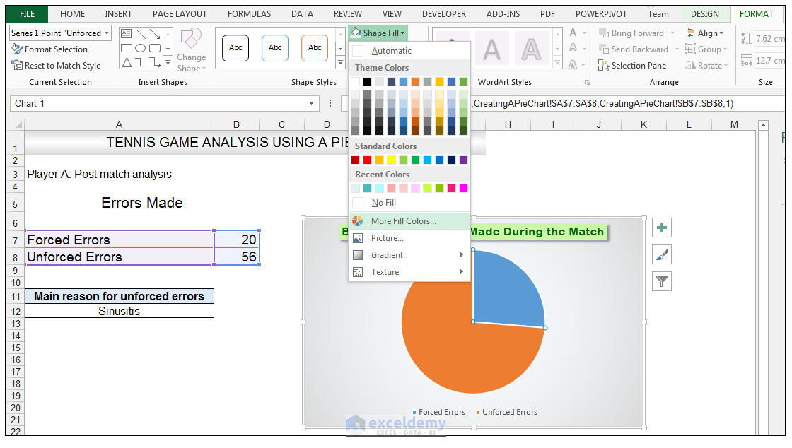
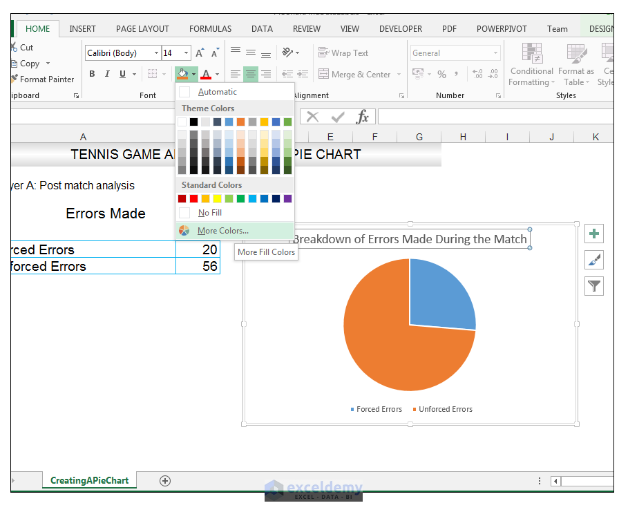
How to add two data labels in excel pie chart. Create two data labels in pie chart? | MrExcel Message Board Aug 30, 2018 — There are 50 pie charts and I don't want to manually adjust each one. Suggestions? Excel Facts. How to Edit Pie Chart in Excel (All Possible Modifications) This will add two tabs named Chart Design and Format in the ribbon. Secondly, go to the Chart Design tab from the ribbon. Subsequently, click on the Change Colors tool. At this time, choose any color you want for your pie chart. Therefore, you will see that you have made edits in your pie chart color successfully according to your choice. How to add or move data labels in Excel chart? - ExtendOffice To add or move data labels in a chart, you can do as below steps: In Excel 2013 or 2016. 1. Click the chart to show the Chart Elements button .. 2. Then click the Chart Elements, and check Data Labels, then you can click the arrow to choose an option about the data labels in the sub menu.See screenshot: How to Create and Format a Pie Chart in Excel - Lifewire To add data labels to a pie chart: Select the plot area of the pie chart. Right-click the chart. Select Add Data Labels . Select Add Data Labels. In this example, the sales for each cookie is added to the slices of the pie chart. Change Colors

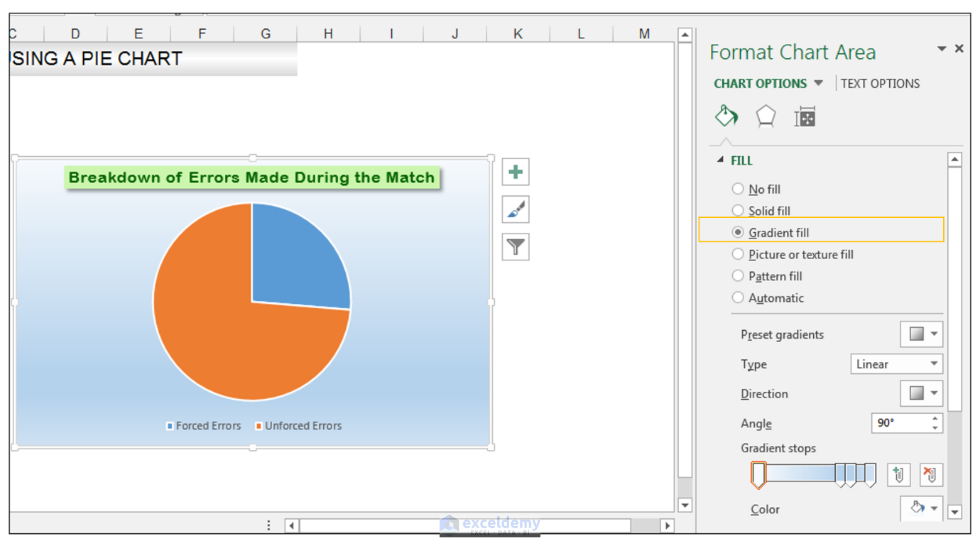
adding decimal places to percentages in pie charts Hello DV_1956. I am V. Arya, Independent Advisor, to work with you on this issue. Right click on your % label - Format Data labels. Beneath Number choose percentage as category. Report abuse. 44 people found this reply helpful. ·. Was this reply helpful? Add or remove data labels in a chart - Microsoft Support Click the data series or chart. To label one data point, after clicking the series, click that data point. In the upper right corner, next to the chart, click Add Chart Element > Data Labels. To change the location, click the arrow, and choose an option. If you want to show your data label inside a text bubble shape, click Data Callout. Creating Pie Chart and Adding/Formatting Data Labels (Excel) Creating Pie Chart and Adding/Formatting Data Labels (Excel) Creating Pie Chart and Adding/Formatting Data Labels (Excel) How to Make a Pie Chart in Excel & Add Rich Data Labels to The Chart! 8) With the one data point still selected, right-click this data point, and select Add Data Label>Add Data Callout as shown below. 9) Select only this data label and right-click and choose Insert Data Label Field as shown below. 10) Select [Cell] Choose Cell from the options.

Adding data labels to a pie chart - OzGrid Free Excel/VBA Help Forum Re: Adding data labels to a pie chart. Thanks again, norie. Really appreciate the help. I tried recording a macro while doing it manually (before my first post). But it didn't record anything about labels, much less making them bold. How to Combine or Group Pie Charts in Microsoft Excel Click on the first chart and then hold the Ctrl key as you click on each of the other charts to select them all. Click Format > Group > Group. All pie charts are now combined as one figure. They will move and resize as one image. Choose Different Charts to View your Data How to Make Pie Chart with Labels both Inside and Outside 1. Right click on the pie chart, click "Add Data Labels"; · 2. Right click on the data label, click "Format Data Labels" in the dialog box; · 3. Pie of Pie Chart in Excel - Inserting, Customizing, Formatting Inserting a Pie of Pie Chart. Let us say we have the sales of different items of a bakery. Below is the data:-. To insert a Pie of Pie chart:-. Select the data range A1:B7. Enter in the Insert Tab. Select the Pie button, in the charts group. Select Pie of Pie chart in the 2D chart section.

Excel charts: add title, customize chart axis, legend and data labels

Thread: Multiple data labels (in separate locations on chart) You can do it in a single chart. Create the chart so it has 2 columns of data. At first only the 1 column of data will be displayed. Move that series to the ...

How to Make a Pie Chart in Excel & Add Rich Data Labels to The Chart!

How to Make a 2010 Excel Pie Chart with Labels Both Inside and Outside This thread is locked. You can follow the question or vote as helpful, but you cannot reply to this thread.

How to Make a Pie Chart in Excel & Add Rich Data Labels to The Chart!

Pie Chart in Excel | How to Create Pie Chart - EDUCBA Step 1: Select the data to go to Insert, click on PIE, and select 3-D pie chart. Step 2: Now, it instantly creates the 3-D pie chart for you. Step 3: Right-click on the pie and select Add Data Labels. This will add all the values we are showing on the slices of the pie.

How to Make a Pie Chart in Excel & Add Rich Data Labels to The Chart!

Edit titles or data labels in a chart - support.microsoft.com On a chart, click one time or two times on the data label that you want to link to a corresponding worksheet cell. The first click selects the data labels for the whole data series, and the second click selects the individual data label. Right-click the data label, and then click Format Data Label or Format Data Labels.

How to Make a Pie Chart in Excel

How to Add Data Labels to an Excel 2010 Chart - dummies Excel provides several options for the placement and formatting of data labels. Use the following steps to add data labels to series in a chart: Click anywhere on the chart that you want to modify. On the Chart Tools Layout tab, click the Data Labels button in the Labels group. A menu of data label placement options appears:

How to Make a Pie Chart in Excel

How to add two data labels for the same data on a pie chart? Consider using two sheets, a "Calculation" sheet and your "Dashboard" sheet. Create your pie graph as usual on the "Dashboard" sheet, but remove all labels. Adjust the colors as desired. On your "Calculation sheet, create the text for your percentage label and your ratio label. For example, the first pie chart charts the data 46 and 76.

4.1 Choosing a Chart Type – Beginning Excel, First Edition

How to Make a Multi-Level Pie Chart in Excel (with Easy Steps) Adding data labels can help us analyze the information precisely. Right-click on the outermost level on the chart and then right-click on the chart. Then from the context menu, click on the Add Data Labels. After clicking on the Add Data Labels, the data labels will show accordingly.

How to insert data labels to a Pie chart in Excel 2013 - YouTube

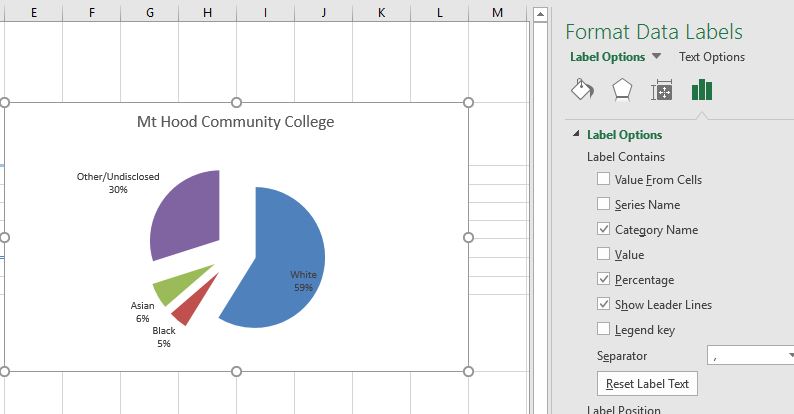
Change the format of data labels in a chart Tip: To switch from custom text back to the pre-built data labels, click Reset Label Text under Label Options. To format data labels, select your chart, and then in the Chart Design tab, click Add Chart Element > Data Labels > More Data Label Options. Click Label Options and under Label Contains, pick the options you want.

34 How To Label A Chart In Excel - Label Ideas 2020

Add data labels and callouts to charts in Excel 365 - EasyTweaks.com Step #1: After generating the chart in Excel, right-click anywhere within the chart and select Add labels . Note that you can also select the very handy option of Adding data Callouts.

32 How To Add Y Axis Label In Excel - Labels Database 2020

How to Add Two Data Labels in Excel Chart (with Easy Steps) Step 1: Create a Chart to Represent Data · Step 2: Add 1st Data Label in Excel Chart · Step 3: Apply 2nd Data Label in Excel Chart · Step 4: Format Data Labels to ...

How to Fake a Two Directional Bar Chart in Excel - Business 2 Community

How to add data labels from different column in an Excel chart? Right click the data series in the chart, and select Add Data Labels > Add Data Labels from the context menu to add data labels. 2. Click any data label to select all data labels, and then click the specified data label to select it only in the chart. 3.

How to Make a Pie Chart in Excel & Add Rich Data Labels to The Chart!

Add a DATA LABEL to ONE POINT on a chart in Excel All the data points will be highlighted. Click again on the single point that you want to add a data label to. Right-click and select ' Add data label '. This is the key step! Right-click again on the data point itself (not the label) and select ' Format data label '. You can now configure the label as required — select the content of ...

Microsoft Excel Tutorials: Add Data Labels to a Pie Chart

How to Make Multiple Pie Charts from One Table (3 Easy Ways) Afterward, go to the Insert tab >> click on Pie Charts. Then, select the 2-D Pie chart. After that, click on the "+" sign to open Chart Elements. Next, turn on Data Labels. Finally, you will get one pie chart from multiple tables in Excel. Practice Section

How to Make a Pie Chart in Excel & Add Rich Data Labels to The Chart!

Pie Chart in Excel - Inserting, Formatting, Filters, Data Labels Click on the Instagram slice of the pie chart to select the instagram. Go to format tab. (optional step) In the Current Selection group, choose data series "hours". This will select all the slices of pie chart. Click on Format Selection Button. As a result, the Format Data Point pane opens.