39 how to add data labels in excel graph
Add Data Points to Existing Chart – Excel & Google Sheets Start with your Graph. Similar to Excel, create a line graph based on the first two columns (Months & Items Sold) Right click on graph; Select Data Range . 3. Select Add Series. 4. Click box for Select a Data Range. 5. Highlight new column and click OK. Final Graph with Single Data Point How to add data labels from different column in an Excel chart? This method will introduce a solution to add all data labels from a different column in an Excel chart at the same time. Please do as follows: 1. Right click the data series in the chart, and select Add Data Labels > Add Data Labels from the context menu to add data labels. 2.
Change the format of data labels in a chart To get there, after adding your data labels, select the data label to format, and then click Chart Elements > Data Labels > More Options. To go to the appropriate area, click one of the four icons ( Fill & Line, Effects, Size & Properties ( Layout & Properties in Outlook or Word), or Label Options) shown here.
How to add data labels in excel graph
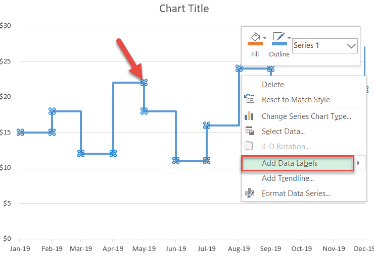
How to Place Labels Directly Through Your Line Graph in Microsoft Excel ... Right-click on top of one of those circular data points. You'll see a pop-up window. Click on Add Data Labels. Your unformatted labels will appear to the right of each data point: Click just once on any of those data labels. You'll see little squares around each data point. Then, right-click on any of those data labels. You'll see a pop-up menu. Excel: How to Create a Bubble Chart with Labels - Statology Step 3: Add Labels. To add labels to the bubble chart, click anywhere on the chart and then click the green plus "+" sign in the top right corner. Then click the arrow next to Data Labels and then click More Options in the dropdown menu: In the panel that appears on the right side of the screen, check the box next to Value From Cells within ... How to add total labels to stacked column chart in Excel? - ExtendOffice Select and right click the new line chart and choose Add Data Labels > Add Data Labels from the right-clicking menu. See screenshot: And now each label has been added to corresponding data point of the Total data series. And the data labels stay at upper-right corners of each column. 5.
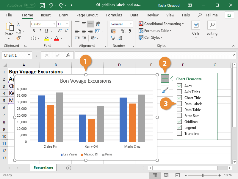
How to add data labels in excel graph. How to add or move data labels in Excel chart? - ExtendOffice 1. Click the chart to show the Chart Elements button . 2. Then click the Chart Elements, and check Data Labels, then you can click the arrow to choose an option about the data labels in the sub menu. See screenshot: How to create a chart with both percentage and value in Excel? Create a chart with both percentage and value in Excel. To solve this task in Excel, please do with the following step by step: 1. Select the data range that you want to create a chart but exclude the percentage column, and then click Insert > Insert Column or Bar Chart > 2-D Clustered Column Chart, see screenshot: 2. How to Add Total Data Labels to the Excel Stacked Bar Chart Apr 03, 2013 · Step 4: Right click your new line chart and select “Add Data Labels” Step 5: Right click your new data labels and format them so that their label position is “Above”; also make the labels bold and increase the font size. Step 6: Right click the line, select “Format Data Series”; in the Line Color menu, select “No line” Step 7 ... How to create Custom Data Labels in Excel Charts - Efficiency 365 Two ways to do it. Click on the Plus sign next to the chart and choose the Data Labels option. We do NOT want the data to be shown. To customize it, click on the arrow next to Data Labels and choose More Options … Unselect the Value option and select the Value from Cells option. Choose the third column (without the heading) as the range.
How to Insert Axis Labels In An Excel Chart | Excelchat We will again click on the chart to turn on the Chart Design tab. We will go to Chart Design and select Add Chart Element. Figure 6 - Insert axis labels in Excel. In the drop-down menu, we will click on Axis Titles, and subsequently, select Primary vertical. Figure 7 - Edit vertical axis labels in Excel. Now, we can enter the name we want ... Edit titles or data labels in a chart - support.microsoft.com On a chart, click one time or two times on the data label that you want to link to a corresponding worksheet cell. The first click selects the data labels for the whole data series, and the second click selects the individual data label. Right-click the data label, and then click Format Data Label or Format Data Labels. HOW TO CREATE A BAR CHART WITH LABELS INSIDE BARS IN EXCEL - simplexCT 7. In the chart, right-click the Series "# Footballers" Data Labels and then, on the short-cut menu, click Format Data Labels. 8. In the Format Data Labels pane, under Label Options selected, set the Label Position to Inside End. 9. Next, in the chart, select the Series 2 Data Labels and then set the Label Position to Inside Base. How to Add Labels to Scatterplot Points in Excel - Statology Step 3: Add Labels to Points. Next, click anywhere on the chart until a green plus (+) sign appears in the top right corner. Then click Data Labels, then click More Options…. In the Format Data Labels window that appears on the right of the screen, uncheck the box next to Y Value and check the box next to Value From Cells.
How to Add Axis Labels in Excel Charts - Step-by-Step (2022) - Spreadsheeto Left-click the Excel chart. 2. Click the plus button in the upper right corner of the chart. 3. Click Axis Titles to put a checkmark in the axis title checkbox. This will display axis titles. 4. Click the added axis title text box to write your axis label. Or you can go to the 'Chart Design' tab, and click the 'Add Chart Element' button ... Add vertical line to Excel chart: scatter plot, bar and line ... May 15, 2019 · In the modern versions of Excel 2013, Excel 2016 and Excel 2019, you can add a horizontal line to a chart with a few clicks, whether it's an average line, target line, benchmark, baseline or whatever. But there is still no easy way to draw a vertical line in Excel graph. However, "no easy way" does not mean no way at all. Excel charts: add title, customize chart axis, legend and data labels Click anywhere within your Excel chart, then click the Chart Elements button and check the Axis Titles box. If you want to display the title only for one axis, either horizontal or vertical, click the arrow next to Axis Titles and clear one of the boxes: Click the axis title box on the chart, and type the text. How to use data labels in a chart - YouTube Excel charts have a flexible system to display values called "data labels". Data labels are a classic example a "simple" Excel feature with a huge range of o...
How to Make & Add Labels on a Graph in Excel : Microsoft Excel Help - YouTube
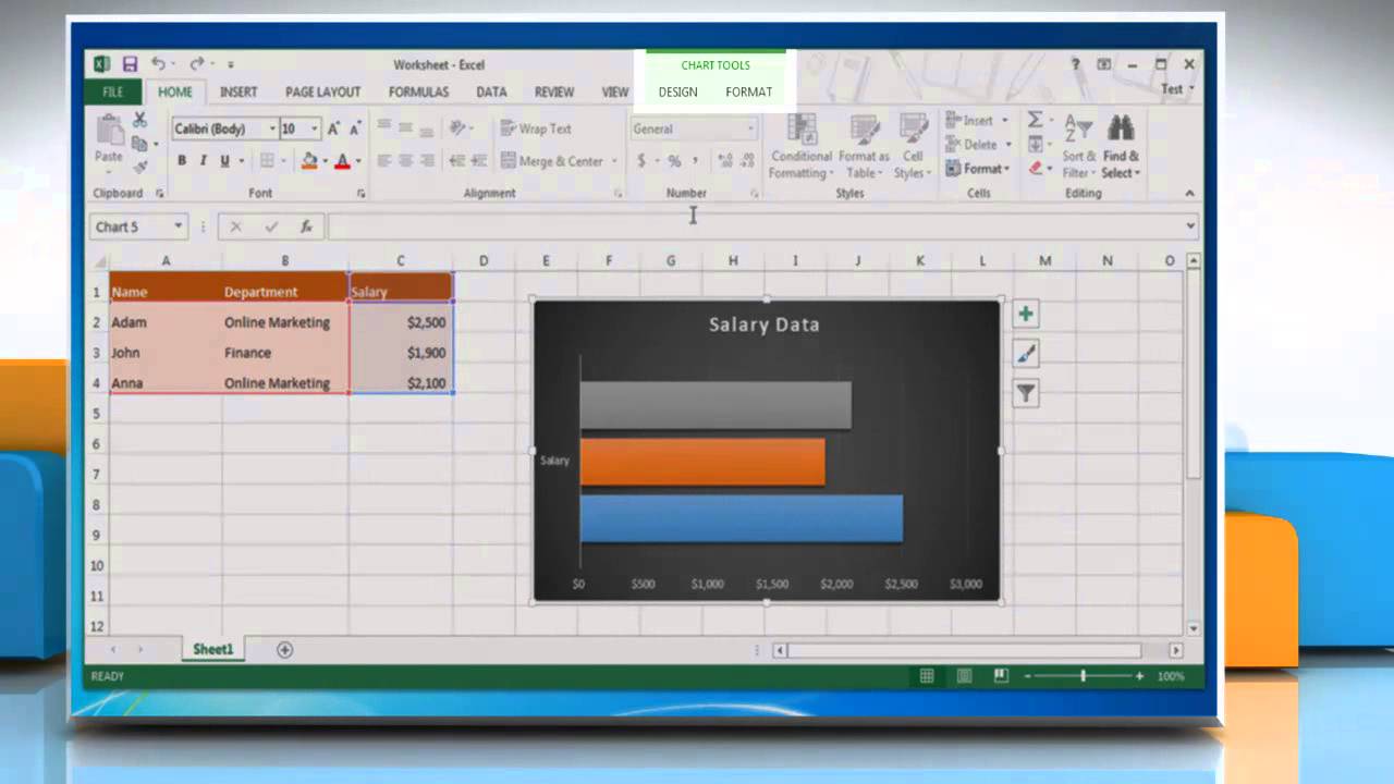
How to add data labels in excel to graph or chart (Step-by-Step) Add data labels to a chart 1. Select a data series or a graph. After picking the series, click the data point you want to label. 2. Click Add Chart Element Chart Elements button > Data Labels in the upper right corner, close to the chart. 3. Click the arrow and select an option to modify the location. 4.

Mapping relationships between people using interactive network chart » Chandoo.org - Learn Excel ...
Add or remove data labels in a chart - support.microsoft.com Add data labels to a chart Click the data series or chart. To label one data point, after clicking the series, click that data point. In the upper right corner, next to the chart, click Add Chart Element > Data Labels. To change the location, click the arrow, and choose an option.
How to Create a Step Chart in Excel - Automate Excel
3 Axis Graph Excel Method: Add a Third Y-Axis - EngineerExcel By default, Excel adds the y-values of the data series. In this case, these were the scaled values, which wouldn’t have been accurate labels for the axis (they would have corresponded directly to the secondary axis). However, in Excel 2013 and later, you can choose a range for the data labels. For this chart, that is the array of unscaled ...
How to Add Axis Labels to a Chart in Excel | CustomGuide
How to add axis label to chart in Excel? - ExtendOffice You can insert the horizontal axis label by clicking Primary Horizontal Axis Title under the Axis Title drop down, then click Title Below Axis, and a text box will appear at the bottom of the chart, then you can edit and input your title as following screenshots shown. 4.

Excel 2013 Tutorial Formatting Data Labels Microsoft Training Lesson 28.6 - YouTube
Add a DATA LABEL to ONE POINT on a chart in Excel Click on the chart line to add the data point to. All the data points will be highlighted. Click again on the single point that you want to add a data label to. Right-click and select ' Add data label ' This is the key step! Right-click again on the data point itself (not the label) and select ' Format data label '.
How to Data Labels in a Bar Graph in Excel 2013 - YouTube
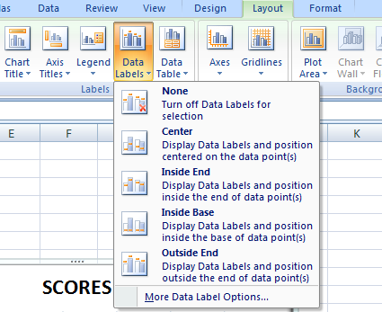
How to Add Data Labels to an Excel 2010 Chart - dummies Excel provides several options for the placement and formatting of data labels. Use the following steps to add data labels to series in a chart: Click anywhere on the chart that you want to modify. On the Chart Tools Layout tab, click the Data Labels button in the Labels group. A menu of data label placement options appears:

Chapter 3 Excel 2007/2010 Charts
How to Add Data Labels in Excel - Excelchat | Excelchat After inserting a chart in Excel 2010 and earlier versions we need to do the followings to add data labels to the chart; Click inside the chart area to display the Chart Tools. Figure 2. Chart Tools Click on Layout tab of the Chart Tools. In Labels group, click on Data Labels and select the position to add labels to the chart. Figure 3.

How to Change Horizontal Axis Labels in Excel 2010 - Solve Your Tech
Add / Move Data Labels in Charts - Excel & Google Sheets Adding Data Labels Click on the graph Select + Sign in the top right of the graph Check Data Labels Change Position of Data Labels Click on the arrow next to Data Labels to change the position of where the labels are in relation to the bar chart Final Graph with Data Labels
How To... Add and Change Chart Titles in Excel 2010 - YouTube
How to Change Excel Chart Data Labels to Custom Values? May 05, 2010 · First add data labels to the chart (Layout Ribbon > Data Labels) Define the new data label values in a bunch of cells, like this: Now, click on any data label. This will select “all” data labels. Now click once again. At this point excel will select only one data label.

How To Use Dynamic Data Labels To Create Interactive Excel Charts
Add a data series to your chart - support.microsoft.com On the worksheet that contains your chart data, in the cells directly next to or below your existing source data for the chart, enter the new data series you want to add. Click the worksheet that contains your chart. Right-click the chart, and then choose Select Data. The Select Data Source dialog box appears on the worksheet that contains the ...

Date Axis in Excel Chart is wrong • AuditExcel.co.za
Custom Chart Data Labels In Excel With Formulas - How To Excel At Excel Follow the steps below to create the custom data labels. Select the chart label you want to change. In the formula-bar hit = (equals), select the cell reference containing your chart label's data. In this case, the first label is in cell E2. Finally, repeat for all your chart laebls.

storytelling with data: May 2013
How To Create Labels In Excel • ganool Axis labels make excel charts easier to understand. Type equals (=) and then the up arrow to enter a formula with a direct cell reference to the first data label. Right click the data series in the chart, and select add data labels > add data labels from the context menu to add data labels.

How to Add Data Labels in Excel - Excelchat | Excelchat
How to Use Cell Values for Excel Chart Labels - How-To Geek Select the chart, choose the "Chart Elements" option, click the "Data Labels" arrow, and then "More Options." Uncheck the "Value" box and check the "Value From Cells" box. Select cells C2:C6 to use for the data label range and then click the "OK" button. The values from these cells are now used for the chart data labels.

How to Add Data Labels in Excel - Excelchat | Excelchat
How to add a line in Excel graph (average line, benchmark ... Sep 12, 2018 · Right-click the selected data point and pick Add Data Label in the context menu: The label will appear at the end of the line giving more information to your chart viewers: Add a text label for the line. To improve your graph further, you may wish to add a text label to the line to indicate what it actually is. Here are the steps for this set up:
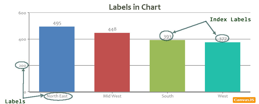
Tutorial on Labels & Index Labels in Chart | CanvasJS JavaScript Charts
how to add data labels into Excel graphs - storytelling with data You can download the corresponding Excel file to follow along with these steps: Right-click on a point and choose Add Data Label. You can choose any point to add a label—I'm strategically choosing the endpoint because that's where a label would best align with my design. Excel defaults to labeling the numeric value, as shown below.

410 How to display percentage labels in pie chart in Excel 2016 - YouTube
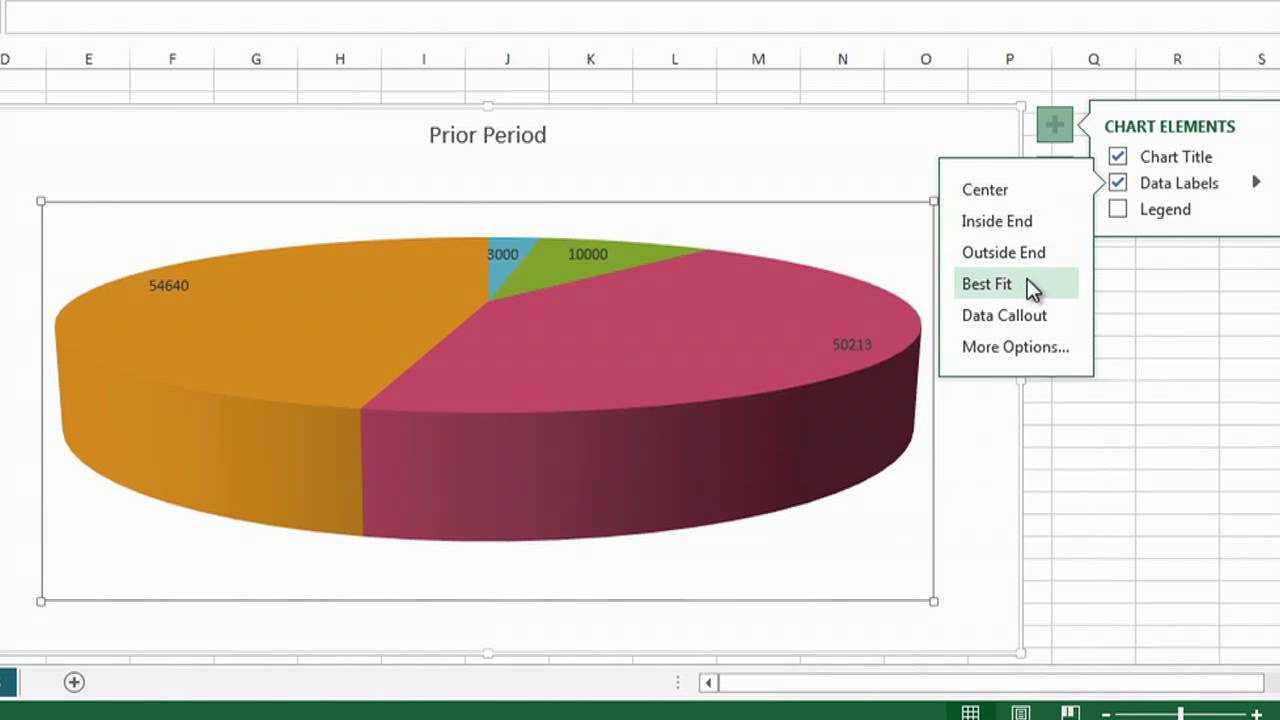
Add data labels and callouts to charts in Excel 365 - EasyTweaks.com Step #1: After generating the chart in Excel, right-click anywhere within the chart and select Add labels . Note that you can also select the very handy option of Adding data Callouts.
how to make a excel graph. - Computer Notes
How to add total labels to stacked column chart in Excel? - ExtendOffice Select and right click the new line chart and choose Add Data Labels > Add Data Labels from the right-clicking menu. See screenshot: And now each label has been added to corresponding data point of the Total data series. And the data labels stay at upper-right corners of each column. 5.

charts - Excel, giving data labels to only the top/bottom X% values - Stack Overflow
Excel: How to Create a Bubble Chart with Labels - Statology Step 3: Add Labels. To add labels to the bubble chart, click anywhere on the chart and then click the green plus "+" sign in the top right corner. Then click the arrow next to Data Labels and then click More Options in the dropdown menu: In the panel that appears on the right side of the screen, check the box next to Value From Cells within ...
Post a Comment for "39 how to add data labels in excel graph"